Torch나 Tensorflow로 짜여진 코드들을 보다보면 einsum() 연산이 포함되어 있는 경우를 볼 수 있습니다. 아주 가끔 보이는 방법이라 보일때마다 해석하는 법을 찾아보고는 했는데, 이번에 살펴보았던 Transformer-XL, XL-Net 구현체(huggingface) 에서는 einsum연산이 자주 등장해서 사용법을 처음부터 정리해보려고 합니다. 이 연산에 대해 잘 설명되어있는 블로그글이 있어, 해당 내용을 많이 참조했습니다.

1. Einsum

torch

torch의 공식문서를 보면 einsum 연산은 Einstein Summation Convention에 따라 연산을 진행하는 방법이라고 나와있습니다. Einstein Notation에 대한 위키피디아 최상단을 보면, 특정 index의 집합에 대한 합 연산(일반적인 \(\sum\limits_{index \space set}\) 연산)을 간결하게 표시하는 방법입니다.

Numpy/Pytorch/Tensorflow은 대부분 동일한 연산들을 지원하는데, 이름과 인자 등에서 미세한 차이가 있을 수 있고, 이들의 차이를 모두 기억하는것은 어렵습니다. einsum 연산을 통해 행렬, 벡터의 내적(Dot products), 외적(Outer products), 전치(Transpose), 행렬곱 등을 일관성있게 표현할 수 있습니다.

참조 블로그의 예시를 통해 Einstein Notation을 만드는 방법을 알아봅니다.

예제 1. Einstein Notation

\(\color{red}{A}\) \(\in \mathbb{R}^{I \times K}\) 와 \(\color{blue}{B}\) \(\in \mathbb{R}^{K \times J}\) 을 이용하여 다음과 같이 계산하여 \(\color{green}{c_j}\) \(\in \mathbb{R}^J\)를 얻습니다.

\[\color{green}{C_{j}}\color{black}{=\sum\limits_{i}\sum\limits_{k}} \color{red}{A_{ik}} \color{blue}{B_{kj}} \color{black}{=} \color{red}{A_{ik}} \color{blue}{B_{kj}}\]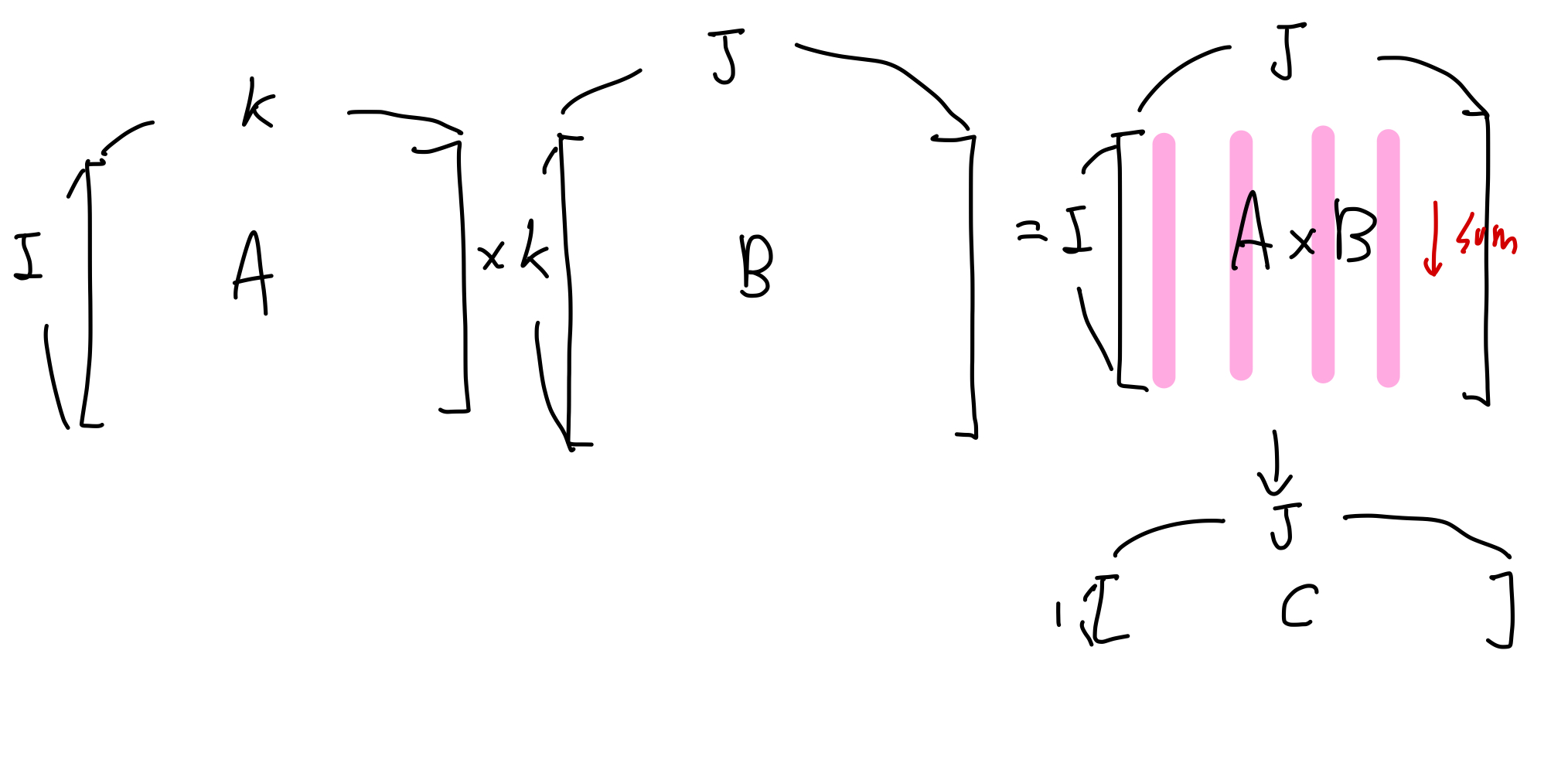

example_1

위 표현식에서 가장 오른쪽에 있는 \(\color{red}{A_{ik}} \color{blue}{B_{kj}}\) 이 Einstein Notation입니다. 이 notation에서는 두 가지 경우에 \(\sum\) 기호(sigma)를 생략하여 표현합니다.

반복적으로 합산되는데 이용되는 index(\(k\))에 관련된 sigma(\(\Sigma\))를 제거합니다.
최종 결과 값(\(C_{j}\))에 명시되지 않은 index(\(i\))에 관련된 sigma(\(\Sigma\))를 제거합니다.

예제 2. 간단한 벡터 연산

이를 이용하여 두 벡터(\(\color{red}{A} \color{black}{,} \color{blue}{B} \color{black}{\in \mathbb{R}^{I}}\))의 내적(dot product)과 외적(outer product)을 Einstein Notation으로 표현해보면 다음과 같습니다.

\[Dot \space product: \color{green}{c} \color{black}{= \sum_i} \color{red}{A_i} \color{blue}{B_i} \color{black}{=} \color{red}{A_i} \color{blue}{B_i}\] \[Outer \space product: \color{green}{C_{i,j}} \color{black}{=} \color{red}{A_i} \color{blue}{B_i} \color{black}{=} \color{red}{A_i} \color{blue}{B_i}\]

예제 3. 복잡한 행렬 연산

조금 더 복잡한 예시를 살펴보면, 3차원의 텐서(\(\color{red}{T}\) \(\in \mathbb{R}^{N \times T \times K}\))의 마지막 차원(\(K\))에 대해 \(\color{blue}{W} \color{black}{\in \mathbb{R}^{K \times Q}}\)를 이용하여 projection 하는 연산을 표현해 보겠습니다. Neural Net에서 이러한 연산은 매우 흔하게 발생합니다. 예를 들어 \(N\)의 배치 크기, \(K\)의 시퀀스 길이 \(K\)의 단어 벡터 임배딩을 다른 차원(\(Q\))으로 projection 시키는 경우를 생각해볼 수 있습니다.

\[\color{green}{C_{ntq}} \color{black}{=\sum_k} \color{red}{T_{ntk}} \color{blue}{W_{kq}} \color{black}{=} \color{red}{T_{ntk}} \color{blue}{W_{kq}}\]

마지막 예제로, 4차원의 텐서(\(\color{red}{T}\) \(\in \mathbb{R}^{N \times T \times K \times M}\))를 이용해 다음과 같은 연산을 진행합니다.

\(\color{red}{T}\)의 3번째 차원을 위에서 정의한 \(\color{blue}{W}\)를 이용해 projection 합니다.
2번째 차원에 대해 합을 진행합니다.
1번째 차원과 마지막 차원을 Transpose합니다.

\[\color{green}{C_{mqn}} \color{black}{=\sum_s\sum_k} \color{red}{T_{ntkm}} \color{blue}{W_{kq}} \color{black}{=} \color{red}{T_{ntkm}} \color{blue}{W_{kq}}\]

transpose는 \(\color{green}{C_{nqm}}\)을 \(\color{green}{C_{mqn}}\)과 같이 index를 바꾸어(\(n \Leftrightarrow m\)) 표현할 수 있습니다.

2. Apply to Numpy, Pytorch, Tensorflow

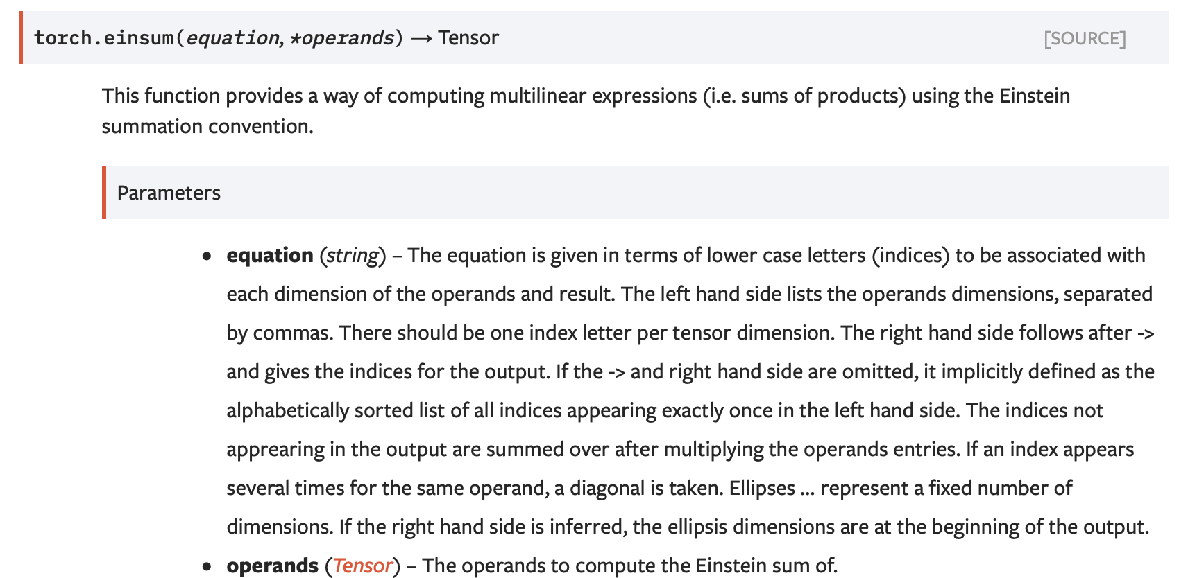
einsum 연산은 numpy(np.einsum), torch(torch.einsum), tensorflow(tf.einsum)과 같이 자주 사용하는 연산 라이브러리에 모두 구현되어 있습니다. 특히 Pytorch와 Tensorflow 에서는 뉴럴넷을 위한 어떤 임의의 연산 그래프 위에서도 back propagation이 가능한 형태로 구현되어 있습니다. 세 경우 모두 einsum(equation, operands)와 같이 인자로 equation 과 operands를 받습니다. 가장 처음 그림에 나와 있는 PyTorch의 문서를 읽어보면 각 인자의 의미는 다음과 같습니다.

equation(string): equation은 operand의 각 index에 대응하는 소문자로 구성되는 식입니다. 식은 "->" 를 기준으로 왼쪽, 오른쪽이 다른 의미를 지닙니다. 왼쪽에는 operand들의 차원을 나열한 것으로 ","를 기준으로 구분됩니다. 오른쪽에는 출력값(output)의 차원 인덱스들을 나타냅니다. 오른쪽은 생략될 수 있는데, 이 경우 왼쪽에서 정확히 한번만 언급된 알파벳들(합의 축이 아닌 알파벳들)을 순서대로 나열한 것으로 내부적으로 정의됩니다. 출력값에 표현되지 않은 인덱스들은 operand들을 곱한 후 해당 인덱스를 기준으로 더해집니다.

위의 행렬 연산 첫번째 예시에서 "ntk,kq->ntq"의 경우, k가 이러한 인덱스에 해당되며, 식으로 나타내면 \(\sum_k \color{red}{T_{ntk}} \color{blue}{W_{kq}}\)과 같이 더해짐을 알 수 있습니다.
operands(Tensor): 해당 연산을 수행할 대상들(operands의 정의) 위의 모든 예시들은 2개의 operand로 구성되어 있지만, 2개 이상에서도 일반화될 수 있습니다.

설명의 예시에서 잠깐 나왔지만 Einetein Notation에서 살펴봤던 notation을 각 함수의 인자인 equation으로 표시할 수 있습니다. 각 operand와 결과 값의 인덱스들로 식을 만들 수 있는데, \(\color{green}{C_{j}}\color{black}{=\sum\limits_{i}\sum\limits_{k}} \color{red}{A_{ik}} \color{blue}{B_{kj}} \color{black}{=} \color{red}{A_{ik}} \color{blue}{B_{kj}}\)의 경우 “\(\color{red}{ik} \color{black}{,} \color{blue}{kj}\) -> \(\color{green}{j}\)“와 같이 나타낼 수 있습니다.

formula

결과적으로 위와 같은 형태로 정형화 하여 이용할 수 있습니다.

2.2 Example

einsum연산을 이용해 표현할 수 있는 예제들을 직접 코드로 구현해보고, np.einsum(), tf.einsum(), torch.einsum()이 모두 같은 결과를 보이는지 확인해 보겠습니다.

Define Check Function

입력 equation과 operands을 이용해 np.einsum(), tf.einsum(), torch.einsum()각각 연산을 진행하고 결과가 같은지 확인하는 함수를 간단하게 구현합니다.

def check_einsum(name: str, equation: str, operands: List[np.ndarray]):
    print(f"{'=' * 10} {name} {'=' * 10}")
    print(f"equation: {equation}\n")

    print(f"Before {name}:\n{operands}\n")

    numpy_result = np.einsum(equation, *operands)
    torch_result = torch.einsum(equation, *[torch.tensor(operand) for operand in operands])
    tf_result = tf.einsum(equation, *[tf.constant(operand) for operand in operands])

    assert np.allclose(numpy_result, torch_result.numpy()), "Numpy result is different from Torch result"
    assert np.allclose(numpy_result, tf_result.numpy()), "Numpy result is different from Tensorflow result"

    print("All results are same!!\n")
    print(f"After {name}:\n{numpy_result}\n")

    return numpy_result

Transpose

\[\color{green}{B_{j, i}} \color{black}{=} \color{red}{A_{i,j}}\]

다음과 같이 2-D텐서에 transpose 연산을 진행하고 결과를 확인합니다.

# 2-D Matrix Transpose
test_matrix = np.random.uniform(size=[2,2])
check_einsum("2-D transpose", "ij->ji", [test_matrix])

========== 2-D transpose ==========
equation: ij->ji

Before 2-D transpose:
[array([[0.8175214 , 0.16426609],
       [0.88842086, 0.56585637]])]

All results are same!!

After 2-D transpose:
[[0.8175214  0.88842086]
 [0.16426609 0.56585637]]

Sum

\[\color{green}{b} \color{black}{= \sum_{i}\sum_{j}} \color{red}{A_{i,j}} \color{black}{=} \color{red}{A_{i,j}}\]

다음과 같이 2-D텐서에 모든 원소들을 합하는 연산을 진행하고 결과를 확인합니다.

# 2-D Matrix Sum
test_matrix = np.arange(4).reshape([2,2])
check_einsum("2-D Sum", "ij->", [test_matrix])

========== 2-D Sum ==========
equation: ij->

Before 2-D Sum:
[array([[0, 1],
       [2, 3]])]

All results are same!!

After 2-D Sum:
6

Column/Row Sum

\[Column \space sum: \color{green}b_j \color{black}{= \sum_i} \color{red}{A_{i,j}} \color{black}{=} \color{red}{A_{i,j}}\] \[Row \space sum: \color{green}b_i \color{black}{= \sum_j} \color{red}{A_{i,j}} \color{black}{=} \color{red}{A_{i,j}}\]

2-D 행렬의 각 열/행을 합치는 연산을 진행하고 결과를 확인합니다.

# Column Sum
test_matrix = np.arange(4).reshape([2,2])
check_einsum("2-D Column Sum", "ij->j", [test_matrix])

# Row Sum
check_einsum("2-D Row Sum", "ij->i", [test_matrix])

========== 2-D Column Sum ==========
equation: ij->j

Before 2-D Column Sum:
[array([[0, 1],
       [2, 3]])]

All results are same!!

After 2-D Column Sum:
[2 4]

========== 2-D Row Sum ==========
equation: ij->i

Before 2-D Row Sum:
[array([[0, 1],
       [2, 3]])]

All results are same!!

After 2-D Row Sum:
[1 5]

Matrix-Matrix(Vector) Multiplication

\[\color{green}{c_i} \color{black}{= \sum_j} \color{red}{A_{i,j}} \color{blue}{b_j} \color{black}{=} \color{red}{A_{i,j}} \color{blue}{b_j}\] \[\color{green}{C_{i,j}}\color{black}{=\sum\limits_{k}} \color{red}{A_{ik}} \color{blue}{B_{kj}} \color{black}{=} \color{red}{A_{ik}} \color{blue}{B_{kj}}\]

2-D 행렬과 2-D행렬(1-D 벡터)의 곱연산을 진행하고 결과를 확인합니다.

test_matrix = np.arange(6).reshape([2,3])
test_vector = np.arange(3)
check_einsum("Matrix-Vector Multiplication", "ij,j->i", [test_matrix, test_vector])
check_einsum("Matrix-Matrix Multiplication", "ik,kj->ij", [test_matrix, test_matrix.T])

========== Matrix-Vector Multiplication ==========
equation: ij,j->i

Before Matrix-Vector Multiplication:
[array([[0, 1, 2],
       [3, 4, 5]]), array([0, 1, 2])]

All results are same!!

After Matrix-Vector Multiplication:
[ 5 14]

========== Matrix-Matrix Multiplication ==========
equation: ik,kj->ij

Before Matrix-Matrix Multiplication:
[array([[0, 1, 2],
       [3, 4, 5]]), array([[0, 3],
       [1, 4],
       [2, 5]])]

All results are same!!

After Matrix-Matrix Multiplication:
[[ 5 14]
 [14 50]]

Dot/Outer/Hadamard Product

\[\text{Dot product}: \color{green}{c} \color{black}{= \sum_i} \color{red}{A_i} \color{blue}{B_i} \color{black}{=} \color{red}{A_i} \color{blue}{B_i}\] \[\text{Outer product}: \color{green}{C_{i,j}} \color{black}{=} \color{red}{A_i} \color{blue}{B_j} \color{black}{=} \color{red}{A_i} \color{blue}{B_j}\] \[\text{Hadamard product}: \color{green}{C_{i,j}} \color{black}{=} \color{red}{A_{i,j}} \color{blue}{B_{i,j}} \color{black}{=} \color{red}{A_{i,j}} \color{blue}{B_{i,j}}\]

1-D 벡터의 Dot/Outer product, 2-D 행렬을 hadamard product연산을 진행하고 결과를 확인합니다.

test_vector_1 = np.arange(3)
test_vector_2 = np.arange(3)

# Dot Product
check_einsum("Dot product", "i,i->", [test_vector_1, test_vector_2])

# Outer Product
check_einsum("Outer product", "i,j->ij", [test_vector_1, test_vector_2])

test_matrix_1 = np.arange(6).reshape([2,3])
test_matrix_2 = np.arange(6).reshape([2,3])

# Hadamard Product
check_einsum("Hadamard product", "ij,ij->ij", [test_matrix_1, test_matrix_2])

========== Dot product ==========
equation: i,i->

Before Dot product:
[array([0, 1, 2]), array([0, 1, 2])]

All results are same!!

After Dot product:
5

========== Outer product ==========
equation: i,j->ij

Before Outer product:
[array([0, 1, 2]), array([0, 1, 2])]

All results are same!!

After Outer product:
[[0 0 0]
 [0 1 2]
 [0 2 4]]

========== Hadamard product ==========
equation: ij,ij->ij

Before Hadamard product:
[array([[0, 1, 2],
       [3, 4, 5]]), array([[0, 1, 2],
       [3, 4, 5]])]

All results are same!!

After Hadamard product:
[[ 0  1  4]
 [ 9 16 25]]

Batch Matrix Multiplication

\[\color{green}{C_{ijl}} \color{black}{=\sum_k} \color{red}{A_{ijk}} \color{blue}{B_{ikl}} \color{black}{=} \color{red}{A_{ijk}} \color{blue}{B_{ikl}}\]

Batch 단위의 행렬곱 연산을 진행하고 결과를 확인합니다. 이 때, torch.bmm()과 연산결과가 일치하는지 또한 확인합니다.

i, j, k, l = 2, 1, 2, 3
test_matrix_1 = np.random.uniform(size=(i,j,k))
test_matrix_2 = np.random.uniform(size=(i,k,l))

einsum_result = check_einsum("Batch Matrix Multiplication", "ijk,ikl->ijl", [test_matrix_1, test_matrix_2])

# coparision between einsum and original bmm

original_bmm = torch.bmm(torch.tensor(test_matrix_1), torch.tensor(test_matrix_2)).numpy()
assert np.all(original_bmm == einsum_result)
print("original bmm result and einsum result are same!")

========== Batch Matrix Multiplication ==========
equation: ijk,ikl->ijl

Before Batch Matrix Multiplication:
[array([[[0.04871888, 0.39235474]],

       [[0.58592502, 0.20879842]]]), array([[[0.53302308, 0.63040016, 0.6521651 ],
        [0.64271892, 0.95364834, 0.25051365]],

       [[0.34683459, 0.30510805, 0.92075663],
        [0.79674854, 0.14313106, 0.10006489]]])]

All results are same!!

After Batch Matrix Multiplication:
[[[0.2781421  0.40488083 0.13006297]]

 [[0.3695789  0.20865598 0.56038774]]]

original bmm result and einsum result are same!

Bilinear Transformation

\[\color{green}{D_{ij}} \color{black}{=\sum_k\sum_l} \color{red}{A_{ik}} \color{purple}{X_{jkl}} \color{blue}{B_{il}} \color{black}{=} \color{red}{A_{ik}} \color{purple}{X_{jkl}} \color{blue}{B_{il}}\]

einsum의 operands 인자는 두 개 이상의 텐서를 입력으로 받을 수 있습니다. 그 예시로 Bilinear Transformation 연산을 진행하고 결과를 확인합니다.torch.nn.functional.bilinear()과 연산결과가 일치하는지 또한 확인합니다.

i,j,k,l = 2,3,2,2
test_matrix_1 = np.random.uniform(size=(i,k))
test_matrix_2 = np.random.uniform(size=(i,l))
X = np.random.uniform(size=(j,k,l))

einsum_result = check_einsum("Bilinear Transformation", "ik,jkl,il->ij", [test_matrix_1, X, test_matrix_2])

original_bilinear = torch.nn.functional.bilinear(torch.tensor(test_matrix_1),
                                                 torch.tensor(test_matrix_2),
                                                 torch.tensor(X)).numpy()
assert np.allclose(original_bilinear, einsum_result)
print("original bilinear result and einsum result are same!")

========== Bilinear Transformation ==========
equation: ik,jkl,il->ij

Before Bilinear Transformation:
[array([[0.35653311, 0.52633733],
       [0.26608957, 0.81076939]]), array([[[0.46743368, 0.17975145],
        [0.08515695, 0.48126152]],

       [[0.18973912, 0.09116181],
        [0.86248519, 0.22003846]],

       [[0.88103597, 0.64415932],
        [0.13718592, 0.12673754]]]), array([[0.62992895, 0.11155462],
       [0.92166012, 0.4382369 ]])]

All results are same!!

After Bilinear Transformation:
[[0.16862208 0.3451204  0.27641856]
 [0.37022668 0.77983982 0.43872821]]

original bilinear result and einsum result are same!

Multi-head Attention(Advanced)

\[\text{MultiHeadAttention}(K,Q,V) = \text{concat}(head_1, head_2, head_3, ...)\] \[head_i = \text{Attention}(QW^Q_i, KW^K_i, VW^V_i)\] \[\text{Attention}(Q,K,V) = \text{softmax}(\frac{QK^{\top}}{\sqrt{d_k}})V\]

“Attention is All you need”의 Multi-head attention을 np.einsum() 을 이용해 구현합니다.

from scipy.special import softmax

def multihead_attention(hidden_states, W_Q, W_K, W_V, num_head):
    batch_size, sequence_length, hidden_size = hidden_states.shape
    assert hidden_size % num_head == 0
    head_hidden_size = hidden_size // num_head

    Q = np.einsum("ijk,kl->ijl", hidden_states, W_Q)   # [batch_size, sequence_length, hidden_size]
    K = np.einsum("ijk,kl->ijl", hidden_states, W_K)   # [batch_size, sequence_length, hidden_size]
    V = np.einsum("ijk,kl->ijl", hidden_states, W_V)   # [batch_size, sequence_length, hidden_size]
    print(f"Q shape: {Q.shape} K shape: {K.shape} V shape: {V.shape}")

    Q = np.reshape(Q, [batch_size, sequence_length, num_head, head_hidden_size]) # [batch_size, sequence_length, num_haed, head_hidden_size]
    K = np.reshape(K, [batch_size, sequence_length, num_head, head_hidden_size]) # [batch_size, sequence_length, num_haed, head_hidden_size]
    V = np.reshape(V, [batch_size, sequence_length, num_head, head_hidden_size]) # [batch_size, sequence_length, num_haed, head_hidden_size]
    print(f"Q shape: {Q.shape} K shape: {K.shape} V shape: {V.shape}")

    Q = np.einsum("ijkl->ikjl", Q)  # [batch_size, num_haed, sequence_length, head_hidden_size]
    K = np.einsum("ijkl->ikjl", K)  # [batch_size, num_haed, sequence_length, head_hidden_size]
    V = np.einsum("ijkl->ikjl", V)  # [batch_size, num_haed, sequence_length, head_hidden_size]
    print(f"Q shape: {Q.shape} K shape: {K.shape} V shape: {V.shape}")

    attention_score = np.einsum("ijkl,ijml->ijkm", Q, K)/np.sqrt(hidden_size)  # [batch_size, num_haed, sequence_length, sequence_length]
    attention_score = softmax(attention_score, axis=3)   # [batch_size, num_haed, sequence_length, sequence_length]
    print(f"Attention score shape: {attention_score.shape}")

    attention_result = np.einsum("ijkl,ijkm->iljm", attention_score, V)   # [batch_size, sequence_length, num_head, head_hidden_size]
    attention_result = np.reshape(attention_result, [batch_size, sequence_length, hidden_size])  # [batch_size, sequence_length, hidden_size]
    print(f"Attention result shape: {attention_result.shape}")

    return attention_result

batch_size, sequence_length, hidden_size, num_head = 2, 10, 16, 8
hidden_states = np.random.uniform(size=(batch_size, sequence_length, hidden_size))

W_K = np.random.uniform(size=(hidden_size, hidden_size))
W_Q = np.random.uniform(size=(hidden_size, hidden_size))
W_V = np.random.uniform(size=(hidden_size, hidden_size))

result = multihead_attention(hidden_states, W_Q, W_K, W_V, num_head)

Q shape: (2, 10, 16) K shape: (2, 10, 16) V shape: (2, 10, 16)
Q shape: (2, 10, 8, 2) K shape: (2, 10, 8, 2) V shape: (2, 10, 8, 2)
Q shape: (2, 8, 10, 2) K shape: (2, 8, 10, 2) V shape: (2, 8, 10, 2)
Attention score shape: (2, 8, 10, 10)
Attention result shape: (2, 10, 16)

위에서 사용한 모든 코드는 Github에 있습니다.

3. 후기

XL-Net/Transformer-XL 구현체를 살펴보다가 einsum()을 자주 사용하는 것 같아서 찾아보게 되었어요. 한국어로 정리된 자료가 없는 것 같아서 “처음부터 찾아보자!”라는 생각으로 시작했는데, 글 하나를 꽉 채웠네요.(처음엔 분량이 적을거라고 예상했는데..) 그래도 좋은 블로그를 찾아서 번역 수준으로 간단하게 끝난 것 같아요. 함수를 처음 봤을 때는 가독성이 좋지 않고 불편할 것 같다고 생각했었는데, 실제로 사용해보니 읽기 불편하지도 않고 tf, torch, numpy에서 모두 동일 메소드로 호환이 된다는 점도 큰 장점인 것 같아요. 물론 실제 학습이나 추론시에는 같은 동작을 하는 다른 메소드들과 시간을 비교해봐야겠지만, 비슷하고 함께 일하는 팀원들이 모두 익숙해 진다면 실제로 써볼만 할 것 같다는 생각이 들었어요. 함수 하나에 너무 많은 시간을 써버렸지만 나름 뿌듯한 시간이였어요. 이제 다시 XL-Net 코드보러 가야겠네요:)

Reference

TIM ROCKTÄSCHEL’s POST
pytorch, numpy, tensorflow Documentation
Ashish Vaswani, Noam Shazeer, Niki Parmar, Jakob Uszkoreit, Llion Jones, Aidan N Gomez, Łukasz Kaiser, and Illia Polosukhin. Attention is all you need. In Advances in neural information processing systems(NeurIPS), 2017.

Einsum 사용하기

Categories

Tags